Quantcast
Channel: 数据库数据恢复服务热线:13764045638 QQ: 47079569
Viewing all 6442 articles
Browse latest View live

MySQL on Docker: Running a MariaDB Galera Cluster without Container Orchestration Tools – Part 1

$
0
0

Container orchestration tools simplify the running of a distributed system, by deploying and redeploying containers and handling any failures that occur. One might need to move applications around, e.g., to handle updates, scaling, or underlying host failures. While this sounds great, it does not always work well with a strongly consistent database cluster like Galera. You can’t just move database nodes around, they are not stateless applications. Also, the order in which you perform operations on a cluster has high significance. For instance, restarting a Galera cluster has to start from the most advanced node, or else you will lose data. Therefore, we’ll show you how to run Galera Cluster on Docker without a container orchestration tool, so you have total control.

In this blog post, we are going to look into how to run a MariaDB Galera Cluster on Docker containers using the standard Docker image on multiple Docker hosts, without the help of orchestration tools like Swarm or Kubernetes. This approach is similar to running a Galera Cluster on standard hosts, but the process management is configured through Docker.

Before we jump further into details, we assume you have installed Docker, disabled SElinux/AppArmor and cleared up the rules inside iptables, firewalld or ufw (whichever you are using). The following are three dedicated Docker hosts for our database cluster:

  • host1.local - 192.168.55.161
  • host2.local - 192.168.55.162
  • host3.local - 192.168.55.163

Multi-host Networking

First of all, the default Docker networking is bound to the local host. Docker Swarm introduces another networking layer called overlay network, which extends the container internetworking to multiple Docker hosts in a cluster called Swarm. Long before this integration came into place, there were many network plugins developed to support this - Flannel, Calico, Weave are some of them.

Here, we are going to use Weave as the Docker network plugin for multi-host networking. This is mainly due to its simplicity to get it installed and running, and support for DNS resolver (containers running under this network can resolve each other's hostname). There are two ways to get Weave running - systemd or through Docker. We are going to install it as a systemd unit, so it's independent from Docker daemon (otherwise, we would have to start Docker first before Weave gets activated).

  1. Download and install Weave:

    $ curl -L git.io/weave -o /usr/local/bin/weave
    $ chmod a+x /usr/local/bin/weave
  2. Create a systemd unit file for Weave:

    $ cat > /etc/systemd/system/weave.service << EOF
    [Unit]
    Description=Weave Network
    Documentation=http://docs.weave.works/weave/latest_release/
    Requires=docker.service
    After=docker.service
    [Service]
    EnvironmentFile=-/etc/sysconfig/weave
    ExecStartPre=/usr/local/bin/weave launch --no-restart $PEERS
    ExecStart=/usr/bin/docker attach weave
    ExecStop=/usr/local/bin/weave stop
    [Install]
    WantedBy=multi-user.target
    EOF
  3. Define IP addresses or hostname of the peers inside /etc/sysconfig/weave:

    $ echo 'PEERS="192.168.55.161 192.168.55.162 192.168.55.163"' > /etc/sysconfig/weave
  4. Start and enable Weave on boot:

    $ systemctl start weave
    $ systemctl enable weave

Repeat the above 4 steps on all Docker hosts. Verify with the following command once done:

$ weave status

The number of peers is what we are looking after. It should be 3:

          ...
          Peers: 3 (with 6 established connections)
          ...

Running a Galera Cluster

Now the network is ready, it's time to fire our database containers and form a cluster. The basic rules are:

  • Container must be created under --net=weave to have multi-host connectivity.
  • Container ports that need to be published are 3306, 4444, 4567, 4568.
  • The Docker image must support Galera. If you'd like to use Oracle MySQL, then get the Codership version. If you'd like Percona's, use this image instead. In this blog post, we are using MariaDB's.

The reasons we chose MariaDB as the Galera cluster vendor are:

  • Galera is embedded into MariaDB, starting from MariaDB 10.1.
  • The MariaDB image is maintained by the Docker and MariaDB teams.
  • One of the most popular Docker images out there.

Bootstrapping a Galera Cluster has to be performed in sequence. Firstly, the most up-to-date node must be started with "wsrep_cluster_address=gcomm://". Then, start the remaining nodes with a full address consisting of all nodes in the cluster, e.g, "wsrep_cluster_address=gcomm://node1,node2,node3". To accomplish these steps using container, we have to do some extra steps to ensure all containers are running homogeneously. So the plan is:

  1. We would need to start with 4 containers in this order - mariadb0 (bootstrap), mariadb2, mariadb3, mariadb1.
  2. Container mariadb0 will be using the same datadir and configdir with mariadb1.
  3. Use mariadb0 on host1 for the first bootstrap, then start mariadb2 on host2, mariadb3 on host3.
  4. Remove mariadb0 on host1 to give way for mariadb1.
  5. Lastly, start mariadb1 on host1.

At the end of the day, you would have a three-node Galera Cluster (mariadb1, mariadb2, mariadb3). The first container (mariadb0) is a transient container for bootstrapping purposes only, using cluster address "gcomm://". It shares the same datadir and configdir with mariadb1 and will be removed once the cluster is formed (mariadb2 and mariadb3 are up) and nodes are synced.

By default, Galera is turned off in MariaDB and needs to be enabled with a flag called wsrep_on (set to ON) and wsrep_provider (set to the Galera library path) plus a number of Galera-related parameters. Thus, we need to define a custom configuration file for the container to configure Galera correctly.

Let's start with the first container, mariadb0. Create a file under /containers/mariadb0/conf.d/my.cnf and add the following lines:

$ mkdir -p /containers/mariadb0/conf.d
$ cat /containers/mariadb0/conf.d/my.cnf
[mysqld]

default_storage_engine          = InnoDB
binlog_format                   = ROW

innodb_flush_log_at_trx_commit  = 0
innodb_flush_method             = O_DIRECT
innodb_file_per_table           = 1
innodb_autoinc_lock_mode        = 2
innodb_lock_schedule_algorithm  = FCFS # MariaDB >10.1.19 and >10.2.3 only

wsrep_on                        = ON
wsrep_provider                  = /usr/lib/galera/libgalera_smm.so
wsrep_sst_method                = xtrabackup-v2

Since the image doesn't come with MariaDB Backup (which is the preferred SST method for MariaDB 10.1 and MariaDB 10.2), we are going to stick with xtrabackup-v2 for the time being.

To perform the first bootstrap for the cluster, run the bootstrap container (mariadb0) on host1:

$ docker run -d \
        --name mariadb0 \
        --hostname mariadb0.weave.local \
        --net weave \
        --publish "3306" \
        --publish "4444" \
        --publish "4567" \
        --publish "4568" \
        $(weave dns-args) \
        --env MYSQL_ROOT_PASSWORD="PM7%cB43$sd@^1" \
        --env MYSQL_USER=proxysql \
        --env MYSQL_PASSWORD=proxysqlpassword \
        --volume /containers/mariadb1/datadir:/var/lib/mysql \
        --volume /containers/mariadb1/conf.d:/etc/mysql/mariadb.conf.d \
        mariadb:10.2.15 \
        --wsrep_cluster_address=gcomm:// \
        --wsrep_sst_auth="root:PM7%cB43$sd@^1" \
        --wsrep_node_address=mariadb0.weave.local

The parameters used in the the above command are:

  • --name, creates the container named "mariadb0",
  • --hostname, assigns the container a hostname "mariadb0.weave.local",
  • --net, places the container in the weave network for multi-host networing support,
  • --publish, exposes ports 3306, 4444, 4567, 4568 on the container to the host,
  • $(weave dns-args), configures DNS resolver for this container. This command can be translated into Docker run as "--dns=172.17.0.1 --dns-search=weave.local.",
  • --env MYSQL_ROOT_PASSWORD, the MySQL root password,
  • --env MYSQL_USER, creates "proxysql" user to be used later with ProxySQL for database routing,
  • --env MYSQL_PASSWORD, the "proxysql" user password,
  • --volume /containers/mariadb1/datadir:/var/lib/mysql, creates /containers/mariadb1/datadir if does not exist and map it with /var/lib/mysql (MySQL datadir) of the container (for bootstrap node, this could be skipped),
  • --volume /containers/mariadb1/conf.d:/etc/mysql/mariadb.conf.d, mounts the files under directory /containers/mariadb1/conf.d of the Docker host, into the container at /etc/mysql/mariadb.conf.d.
  • mariadb:10.2.15, uses MariaDB 10.2.15 image from here,
  • --wsrep_cluster_address, Galera connection string for the cluster. "gcomm://" means bootstrap. For the rest of the containers, we are going to use a full address instead.
  • --wsrep_sst_auth, authentication string for SST user. Use the same user as root,
  • --wsrep_node_address, the node hostname, in this case we are going to use the FQDN provided by Weave.

The bootstrap container contains several key things:

  • The name, hostname and wsrep_node_address is mariadb0, but it uses the volumes of mariadb1.
  • The cluster address is "gcomm://"
  • There are two additional --env parameters - MYSQL_USER and MYSQL_PASSWORD. This parameters will create additional user for our proxysql monitoring purpose.

Verify with the following command:

$ docker ps
$ docker logs -f mariadb0

Once you see the following line, it indicates the bootstrap process is completed and Galera is active:

2018-05-30 23:19:30 139816524539648 [Note] WSREP: Synchronized with group, ready for connections

Create the directory to load our custom configuration file in the remaining hosts:

$ mkdir -p /containers/mariadb2/conf.d # on host2
$ mkdir -p /containers/mariadb3/conf.d # on host3

Then, copy the my.cnf that we've created for mariadb0 and mariadb1 to mariadb2 and mariadb3 respectively:

$ scp /containers/mariadb1/conf.d/my.cnf /containers/mariadb2/conf.d/ # on host1
$ scp /containers/mariadb1/conf.d/my.cnf /containers/mariadb3/conf.d/ # on host1

Next, create another 2 database containers (mariadb2 and mariadb3) on host2 and host3 respectively:

$ docker run -d \
        --name ${NAME} \
        --hostname ${NAME}.weave.local \
        --net weave \
        --publish "3306:3306" \
        --publish "4444" \
        --publish "4567" \
        --publish "4568" \
        $(weave dns-args) \
        --env MYSQL_ROOT_PASSWORD="PM7%cB43$sd@^1" \
        --volume /containers/${NAME}/datadir:/var/lib/mysql \
        --volume /containers/${NAME}/conf.d:/etc/mysql/mariadb.conf.d \
        mariadb:10.2.15 \
    
--wsrep_cluster_address=gcomm://mariadb0.weave.local,mariadb1.weave.local,mariadb2.weave.local,mariadb3.weave.local \
        --wsrep_sst_auth="root:PM7%cB43$sd@^1" \
        --wsrep_node_address=${NAME}.weave.local

** Replace ${NAME} with mariadb2 or mariadb3 respectively.

However, there is a catch. The entrypoint script checks the mysqld service in the background after database initialization by using MySQL root user without password. Since Galera automatically performs synchronization through SST or IST when starting up, the MySQL root user password will change, mirroring the bootstrapped node. Thus, you would see the following error during the first start up:

018-05-30 23:27:13 140003794790144 [Warning] Access denied for user 'root'@'localhost' (using password: NO)
MySQL init process in progress…
MySQL init process failed.

The trick is to restart the failed containers once more, because this time, the MySQL datadir would have been created (in the first run attempt) and it would skip the database initialization part:

$ docker start mariadb2 # on host2
$ docker start mariadb3 # on host3

Once started, verify by looking at the following line:

$ docker logs -f mariadb2
…
2018-05-30 23:28:39 139808069601024 [Note] WSREP: Synchronized with group, ready for connections

At this point, there are 3 containers running, mariadb0, mariadb2 and mariadb3. Take note that mariadb0 is started using the bootstrap command (gcomm://), which means if the container is automatically restarted by Docker in the future, it could potentially become disjointed with the primary component. Thus, we need to remove this container and replace it with mariadb1, using the same Galera connection string with the rest and use the same datadir and configdir with mariadb0.

First, stop mariadb0 by sending SIGTERM (to ensure the node is going to be shutdown gracefully):

$ docker kill -s 15 mariadb0

Then, start mariadb1 on host1 using similar command as mariadb2 or mariadb3:

$ docker run -d \
        --name mariadb1 \
        --hostname mariadb1.weave.local \
        --net weave \
        --publish "3306:3306" \
        --publish "4444" \
        --publish "4567" \
        --publish "4568" \
        $(weave dns-args) \
        --env MYSQL_ROOT_PASSWORD="PM7%cB43$sd@^1" \
        --volume /containers/mariadb1/datadir:/var/lib/mysql \
        --volume /containers/mariadb1/conf.d:/etc/mysql/mariadb.conf.d \
        mariadb:10.2.15 \
    
--wsrep_cluster_address=gcomm://mariadb0.weave.local,mariadb1.weave.local,mariadb2.weave.local,mariadb3.weave.local \
        --wsrep_sst_auth="root:PM7%cB43$sd@^1" \
        --wsrep_node_address=mariadb1.weave.local

This time, you don't need to do the restart trick because MySQL datadir already exists (created by mariadb0). Once the container is started, verify the cluster size is 3, the status must be in Primary and the local state is synced:

$ docker exec -it mariadb3 mysql -uroot "-pPM7%cB43$sd@^1" -e 'select variable_name, variable_value from information_schema.global_status where variable_name in ("wsrep_cluster_size", "wsrep_local_state_comment", "wsrep_cluster_status", "wsrep_incoming_addresses")'
+---------------------------+-------------------------------------------------------------------------------+
| variable_name             | variable_value                                                                |
+---------------------------+-------------------------------------------------------------------------------+
| WSREP_CLUSTER_SIZE        | 3                                                                             |
| WSREP_CLUSTER_STATUS      | Primary                                                                       |
| WSREP_INCOMING_ADDRESSES  | mariadb1.weave.local:3306,mariadb3.weave.local:3306,mariadb2.weave.local:3306 |
| WSREP_LOCAL_STATE_COMMENT | Synced                                                                        |
+---------------------------+-------------------------------------------------------------------------------+

At this point, our architecture is looking something like this:

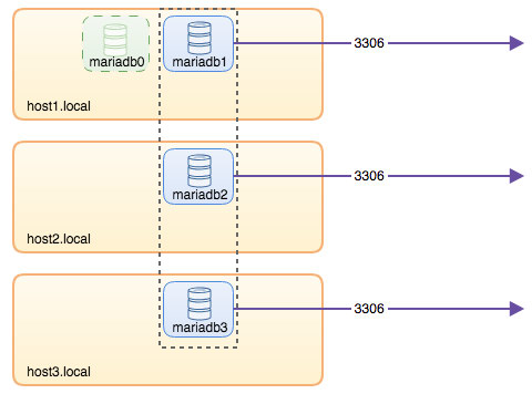
Although the run command is pretty long, it well describes the container's characteristics. It's probably a good idea to wrap the command in a script to simplify the execution steps, or use a compose file instead.

Database Routing with ProxySQL

Now we have three database containers running. The only way to access to the cluster now is to access the individual Docker host’s published port of MySQL, which is 3306 (map to 3306 to the container). So what happens if one of the database containers fails? You have to manually failover the client's connection to the next available node. Depending on the application connector, you could also specify a list of nodes and let the connector do the failover and query routing for you (Connector/J, PHP mysqlnd). Otherwise, it would be a good idea to unify the database resources into a single resource, that can be called a service.

This is where ProxySQL comes into the picture. ProxySQL can act as the query router, load balancing the database connections similar to what "Service" in Swarm or Kubernetes world can do. We have built a ProxySQL Docker image for this purpose and will maintain the image for every new version with our best effort.

Before we run the ProxySQL container, we have to prepare the configuration file. The following is what we have configured for proxysql1. We create a custom configuration file under /containers/proxysql1/proxysql.cnf on host1:

$ cat /containers/proxysql1/proxysql.cnf
datadir="/var/lib/proxysql"
admin_variables=
{
        admin_credentials="admin:admin"
        mysql_ifaces="0.0.0.0:6032"
        refresh_interval=2000
}
mysql_variables=
{
        threads=4
        max_connections=2048
        default_query_delay=0
        default_query_timeout=36000000
        have_compress=true
        poll_timeout=2000
        interfaces="0.0.0.0:6033;/tmp/proxysql.sock"
        default_schema="information_schema"
        stacksize=1048576
        server_version="5.1.30"
        connect_timeout_server=10000
        monitor_history=60000
        monitor_connect_interval=200000
        monitor_ping_interval=200000
        ping_interval_server=10000
        ping_timeout_server=200
        commands_stats=true
        sessions_sort=true
        monitor_username="proxysql"
        monitor_password="proxysqlpassword"
}
mysql_servers =
(
        { address="mariadb1.weave.local" , port=3306 , hostgroup=10, max_connections=100 },
        { address="mariadb2.weave.local" , port=3306 , hostgroup=10, max_connections=100 },
        { address="mariadb3.weave.local" , port=3306 , hostgroup=10, max_connections=100 },
        { address="mariadb1.weave.local" , port=3306 , hostgroup=20, max_connections=100 },
        { address="mariadb2.weave.local" , port=3306 , hostgroup=20, max_connections=100 },
        { address="mariadb3.weave.local" , port=3306 , hostgroup=20, max_connections=100 }
)
mysql_users =
(
        { username = "sbtest" , password = "password" , default_hostgroup = 10 , active = 1 }
)
mysql_query_rules =
(
        {
                rule_id=100
                active=1
                match_pattern="^SELECT .* FOR UPDATE"
                destination_hostgroup=10
                apply=1
        },
        {
                rule_id=200
                active=1
                match_pattern="^SELECT .*"
                destination_hostgroup=20
                apply=1
        },
        {
                rule_id=300
                active=1
                match_pattern=".*"
                destination_hostgroup=10
                apply=1
        }
)
scheduler =
(
        {
                id = 1
                filename = "/usr/share/proxysql/tools/proxysql_galera_checker.sh"
                active = 1
                interval_ms = 2000
                arg1 = "10"
                arg2 = "20"
                arg3 = "1"
                arg4 = "1"
                arg5 = "/var/lib/proxysql/proxysql_galera_checker.log"
        }
)

The above configuration will:

  • configure two host groups, the single-writer and multi-writer group, as defined under "mysql_servers" section,
  • send reads to all Galera nodes (hostgroup 20) while write operations will go to a single Galera server (hostgroup 10),
  • schedule the proxysql_galera_checker.sh,
  • use monitor_username and monitor_password as the monitoring credentials created when we first bootstrapped the cluster (mariadb0).

Copy the configuration file to host2, for ProxySQL redundancy:

$ mkdir -p /containers/proxysql2/ # on host2
$ scp /containers/proxysql1/proxysql.cnf /container/proxysql2/ # on host1

Then, run the ProxySQL containers on host1 and host2 respectively:

$ docker run -d \
        --name=${NAME} \
        --publish 6033 \
        --publish 6032 \
        --restart always \
        --net=weave \
        $(weave dns-args) \
        --hostname ${NAME}.weave.local \
        -v /containers/${NAME}/proxysql.cnf:/etc/proxysql.cnf \
        -v /containers/${NAME}/data:/var/lib/proxysql \
        severalnines/proxysql

** Replace ${NAME} with proxysql1 or proxysql2 respectively.

We specified --restart=always to make it always available regardless of the exit status, as well as automatic startup when Docker daemon starts. This will make sure the ProxySQL containers act like a daemon.

Verify the MySQL servers status monitored by both ProxySQL instances (OFFLINE_SOFT is expected for the single-writer host group):

$ docker exec -it proxysql1 mysql -uadmin -padmin -h127.0.0.1 -P6032 -e 'select hostgroup_id,hostname,status from mysql_servers'
+--------------+----------------------+--------------+
| hostgroup_id | hostname             | status       |
+--------------+----------------------+--------------+
| 10           | mariadb1.weave.local | ONLINE       |
| 10           | mariadb2.weave.local | OFFLINE_SOFT |
| 10           | mariadb3.weave.local | OFFLINE_SOFT |
| 20           | mariadb1.weave.local | ONLINE       |
| 20           | mariadb2.weave.local | ONLINE       |
| 20           | mariadb3.weave.local | ONLINE       |
+--------------+----------------------+--------------+

At this point, our architecture is looking something like this:

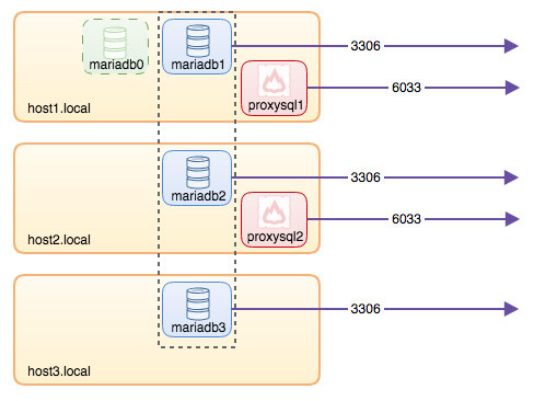
All connections coming from 6033 (either from the host1, host2 or container's network) will be load balanced to the backend database containers using ProxySQL. If you would like to access an individual database server, use port 3306 of the physical host instead. There is no virtual IP address as single endpoint configured for the ProxySQL service, but we could have that by using Keepalived, which is explained in the next section.

Virtual IP Address with Keepalived

Since we configured ProxySQL containers to be running on host1 and host2, we are going to use Keepalived containers to tie these hosts together and provide virtual IP address via the host network. This allows a single endpoint for applications or clients to connect to the load balancing layer backed by ProxySQL.

As usual, create a custom configuration file for our Keepalived service. Here is the content of /containers/keepalived1/keepalived.conf:

vrrp_instance VI_DOCKER {
   interface ens33               # interface to monitor
   state MASTER
   virtual_router_id 52          # Assign one ID for this route
   priority 101
   unicast_src_ip 192.168.55.161
   unicast_peer {
      192.168.55.162
   }
   virtual_ipaddress {
      192.168.55.160             # the virtual IP
}

Copy the configuration file to host2 for the second instance:

$ mkdir -p /containers/keepalived2/ # on host2
$ scp /containers/keepalived1/keepalived.conf /container/keepalived2/ # on host1

Change the priority from 101 to 100 inside the copied configuration file on host2:

$ sed -i 's/101/100/g' /containers/keepalived2/keepalived.conf

**The higher priority instance will hold the virtual IP address (in this case is host1), until the VRRP communication is interrupted (in case host1 goes down).

Then, run the following command on host1 and host2 respectively:

$ docker run -d \
        --name=${NAME} \
        --cap-add=NET_ADMIN \
        --net=host \
        --restart=always \
        --volume /containers/${NAME}/keepalived.conf:/usr/local/etc/keepalived/keepalived.conf \ osixia/keepalived:1.4.4

** Replace ${NAME} with keepalived1 and keepalived2.

The run command tells Docker to:

  • --name, create a container with
  • --cap-add=NET_ADMIN, add Linux capabilities for network admin scope
  • --net=host, attach the container into the host network. This will provide virtual IP address on the host interface, ens33
  • --restart=always, always keep the container running,
  • --volume=/containers/${NAME}/keepalived.conf:/usr/local/etc/keepalived/keepalived.conf, map the custom configuration file for container's usage.

After both containers are started, verify the virtual IP address existence by looking at the physical network interface of the MASTER node:

$ ip a | grep ens33
2: ens33: <BROADCAST,MULTICAST,UP,LOWER_UP> mtu 1500 qdisc pfifo_fast state UP qlen 1000
    inet 192.168.55.161/24 brd 192.168.55.255 scope global ens33
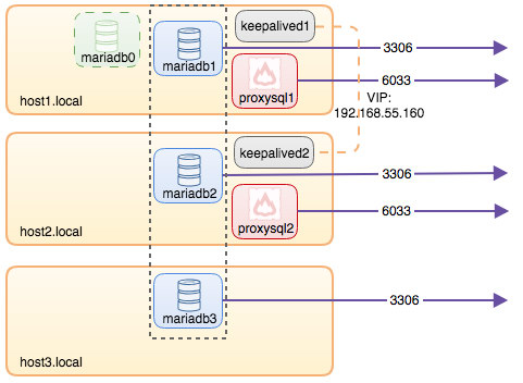
    inet 192.168.55.160/32 scope global ens33

The clients and applications may now use the virtual IP address, 192.168.55.160 to access the database service. This virtual IP address exists on host1 at this moment. If host1 goes down, keepalived2 will take over the IP address and bring it up on host2. Take note that the configuration for this keepalived does not monitor the ProxySQL containers. It only monitors the VRRP advertisement of the Keepalived peers.

At this point, our architecture is looking something like this:

Summary

So, now we have a MariaDB Galera Cluster fronted by a highly available ProxySQL service, all running on Docker containers.

In part two, we are going to look into how to manage this setup. We’ll look at how to perform operations like graceful shutdown, bootstrapping, detecting the most advanced node, failover, recovery, scaling up/down, upgrades, backup and so on. We will also discuss the pros and cons of having this setup for our clustered database service.

Happy containerizing!


Benchmarking the Read Backup feature in the NDB storage engine

$
0
0
Read Backup was a new feature in MySQL Cluster 7.5. When MySQL
Cluster 7.5 was released I was already busily engaged in working
on the partial LCP feature we now released in 7.6. So I had not
much time producing benchmarks showing the impact of the
Read Backup feature.

Read Backup means that committed reads in NDB can use the backup
replicas as well. In NDB tables reads are already directed towards
the primary replica. The reason is that MySQL Cluster wants to
ensure that applications can trust that a reader can see his own
updates. Many modern NoSQL DBMSs lack this feature since they are
using eventual replication and a very flexible scheduling of which
replicas to read. NDB provides a stronger consistency guarantee
in that all applications can see their own updates and replication
is synchronous.

The reason that reading using a backup replica can fail to see its own
changes in NDB is that we release the locks on the primary replica first,
next we deliver the committed message to the application and last
we release the locks on the backup. This means that reading a
backup replica using committed read (reads the latest committed row without
locks) can only be guaranteed to see its own updates if it reads the
primary replica.

With tables that have the Read Backup feature we will delay the
sending of the committed message to the application until all rows
have been unlocked. This means that we can safely read any replica
for those tables and still see our own updates.

Setting the Read Backup feature for a table can either be set through
a special syntax using the COMMENT in the CREATE TABLE statement. A
much easier and likely more useful approach is to set the
ndb_read_backup configuration variable in the MySQL Server to 1. This
means that all tables in this MySQL Server will be created with the
Read Backup feature. Similarly there is a similar feature for ensuring
that all tables are created with the fully replicated feature. In this
case the configuration variable ndb_fully_replicated is set to 1. In
MySQL Cluster 7.6 none of these configuration variables are enabled by
default. But for SQL applications it is a good to always enable the
read backup feature and for applications that focus on read scalability
with fairly limited size of the data, the fully replicated feature can
also be enabled.

Fully replicated tables have a replica in each data node and any replica
can be read for committed reads.

The benchmark we present here is performed in a setup with the optimal
network architecture. It is two machines where the MySQL Server and the
NDB data node can be colocated and the network between the nodes is
using an Infiniband network. This means that in most every real case the
impact of using read backup in a colocated scenario is even bigger.

In this scenario the extra delay to go over the network is fairly small,
thus the impact of low concurrency is fairly small, but the extra overhead
of going over the network a lot shows its impact on higher concurrency and
grows all the way up to 30%.

MySQL Cluster 7.6 and the thread pool

$
0
0
Looking at the graphs in the previous blog post one can see that
MySQL Cluster 7.6 using the shared memory transporter can improve
performance at very high thread counts by more than 100%. Still
the performance is still dropping fairly significantly moving from
512 to 1536 threads. The MySQL Server using the NDB transporter
scales very well on all sorts of architectures and using very many
cores. But I have noted that when the number of connections goes
beyond some limit (in my benchmarks usually around 512 threads),
the performance starts to drop.

Actually in the commercial version of MySQL Cluster help is available
to resolve this problem. The thread pool was developed by me and a team
of performance experts to ensure that MySQL using InnoDB would have
the same performance even with massive amounts of threads hitting at the
MySQL server. It still works for this purpose. I have never mentioned
the use of thread pool for MySQL Cluster before, but the fact of the matter
is that it works perfectly fine to use the thread pool in combination
with MySQL Cluster.

There is one limitation in the current thread pool implementation. The maximum
number of thread groups are 64. This limit was set since MySQL didn't scale
beyond this number using InnoDB in those days. NDB is a distributed engine,
so it works a bit differently for NDB compared to InnoDB. It would be possible
to make the integration of the thread pool and NDB a bit tighter. But even with
the current implementation NDB can be used perfectly fine with the thread pool.

The limit 64 means that it won't really be so useful to use the thread pool and
NDB in combination with MySQL servers that use more than 16 CPUs.
The graph above show how the thread pool compares to the performance of
MySQL Cluster 7.6 on a small MySQL Server. It loses 1-2% on low thread
counts, but it continues to deliver good results even when passing the 512 thread limit.

The graph below shows how MySQL Cluster 7.6.6 using the thread pool compares to
MySQL Cluster 7.5.9 without thread pool. We see the usual linear curve at
high concurrency for the thread pool, in this case however it is limited by
the 64 thread groups since the setup in this case have access to 30 CPUs using
one cluster connection. I did some experiments where I moved the limit of 64
up a bit (a minor change). The performance for most experiments has a
good setting with thread pool size set to 128 and in this case the performance
actually increases a small bit as the number of threads increase.


Oracle 12cR1&11gR2-Concurrent statistics gathering

$
0
0

oracle 11.2统计信息推出了新的参数”CONCURRENT”,但是在11g的官方文档中没有列出来,只到12.1才被列入,所以很多人认为这个是12c的新特性,但是11.2.0.2版本之后就可以使用了,该参数的主要作用是同时收集多个表和表分区的统计信息。它使用的主要是job scheduler, advanced queuing and resource manager来结合操作。系统如果资源很空闲,并发收集统计信息可以减少收集的时间。同时还有一个很好的使用场景,假设你有一个很大的分区表,你需要收集所有该分区上的统计信息,DBA一般会编写脚,使用dbms_stats.gather_table_stats()中的tabname和partname参数并行执行针对单个分区统计信息收集作业。这是人为的并行的方式。而12.1直接推出了并行收集,那么我们可以使用这种新选项来操作。
首先你需要启动并行收集,通过SET_GLOBAL_PREFS方法对全局进行设置。接下来我们创建一个较大的分区表,插入大量数据。然后观察表的CONCURRENT属性是否为True,如果为True就代表这个表可以进行并发收集。

begin
DBMS_STATS.SET_GLOBAL_PREFS('CONCURRENT','TRUE');
end;
/
create table test1
(
id1 number,
id2 varchar2(9)
)
partition by range(id1)
(
partition p1 values less than(10000000),
partition p2 values less than(20000000),
partition p3 values less than(30000000),
partition p4 values less than(40000001)
);

begin
for i in 0..40000000
loop
insert into test1 values(i, 'a'||i);
end loop;
commit;
end;
/

SQL> insert into test1 select /*+parallel(a,4) */ * from test1 a;
40000001 rows created.

SQL> commit;
Commit complete.

这里我们创建了test1表,一共有四个分区,然后我们造了80000000行数据。因为全局设置了CONCURRENT为true,所以我单独的查这张表的CONCURRENT属性也是为true的。

SQL> select dbms_stats.get_prefs('CONCURRENT','SYS','TEST1') from dual;

DBMS_STATS.GET_PREFS('CONCURRENT','SYS','TEST1')
--------------------------------------------------------------------------------
TRUE

SQL> select partition_name, num_rows, sample_size, last_analyzed from user_tab_partitions where table_name = 'TEST1';

PARTITION_NAME NUM_ROWS SAMPLE_SIZE LAST_ANAL
---------------------------------------- ---------- ----------- ---------
P1
P2
P3
P4

SQL> select partition_name, bytes/1024/1024 MB from user_segments where segment_name = 'TEST1';

PARTITION_NAME MB
---------------------------------------- ----------
P1 456
P2 432
P3 456
P4 456

然后开始收集统计信息,这里我开了4个并行。这里需要注意的是,前面我们说过,我们开启用CONCURRENT属性,Oracle是通过job scheduler, advanced queuing and resource manager来结合实现的,所以这里我们的job_queue_processes参数至少是要大于4才行。这里我们还需要搞清楚一个概念,现在我们做的是并发收集统计信息。而不是并行收集统计信息,具体的意思就是,我开了四个并发job在同时进行收集,如果我的这些分区下面还有很多子分区,那么我就可以在并发里面开并行。那么要实现在并发里面在开并行就需要将参数parallel_adaptive_multi_user设置成flase。默认这个参数在11g中就是flase的。这个参数的含义是启用自适应算法,提高使用并行执行的多用户环境中的性能。
关于这个参数的相关设置可以参考Oracle官方的博客,作者是:Guest Author,在并发job任务里面开并行就得关闭这个参数。
If you plan to execute the concurrent statistics gathering jobs in parallel you should disable the parallel adaptive multi-user initialization parameter. That is;
Alter system set parallel_adaptive_multi_user=false;当然这篇文章的博主还建议设置资源管理器,使用并行语句排队。我们这里先不设置resource manager实验并行语句排队,我们直接开始收集,并通过另外一个窗口进行观察。

dbms_stats.gather_table_stats('SYS', 'TEST1', degree=>4)

SQL> select OWNER,JOB_NAME,STATE,SCHEDULE_NAME,COMMENTS from dba_scheduler_jobs where job_class like 'CONC%';

OWNER JOB_NAME STATE SCHEDULE_NAME COMMENTS
------------------------------ ------------------------------ --------------- -------------------- ----------------------------------------
SYS ST$T342_5 RUNNING SYS.TEST1.
SYS ST$T342_4 RUNNING SYS.TEST1.P4
SYS ST$T342_3 RUNNING SYS.TEST1.P3
SYS ST$T342_2 RUNNING SYS.TEST1.P2
SYS ST$T342_1 RUNNING SYS.TEST1.P1

可以看到开启了五个任务在执行,一个是收集表,四个是在收集分区的。同时为了进一步看清楚它做了什么,我们可以通过DBMS_METADATA.GET_DDL来获取DDL。不过很奇怪,我的数据库版本死活都没办法在SYS用户下取出DDL。一直都会报ORA-31603错误,按照MOS上的文档做也解决不了。

Enter value for 1: ST$T339_3
old 1: SELECT DBMS_METADATA.GET_DDL('PROCOBJ', '&1') from dual
new 1: SELECT DBMS_METADATA.GET_DDL('PROCOBJ', 'ST$T339_3') from dual
ERROR:
ORA-31603: object "ST$T339_3" of type PROCOBJ not found in schema "SYS"
ORA-06512: at "SYS.DBMS_METADATA", line 5805
ORA-06512: at "SYS.DBMS_METADATA", line 8344
ORA-06512: at line 1

为了解决这个问题,查了好久,终于发现可以使用dbms_scheduler.copy_job的办法解决。复制到其他的用户下面,然后再执行GET_DDL就彻底的弄出来dbms_scheduler创建的JOB代码。

SQL> exec dbms_scheduler.copy_job('SYS.ST$T342_1','AAA.ST$T342_1');
PL/SQL procedure successfully completed.

SQL> SELECT DBMS_METADATA.GET_DDL('PROCOBJ', '&1','AAA') from dual;
Enter value for 1: ST$T342_1
old 1: SELECT DBMS_METADATA.GET_DDL('PROCOBJ', '&1','AAA') from dual
new 1: SELECT DBMS_METADATA.GET_DDL('PROCOBJ', 'ST$T342_1','AAA') from dual

DBMS_METADATA.GET_DDL('PROCOBJ','ST$T342_1','AAA')
--------------------------------------------------------------------------------
BEGIN
dbms_scheduler.create_job('"ST$T342_1"',
job_type=>'PLSQL_BLOCK', job_action=>
'declare context dbms_stats.CContext := dbms_stats.CContext(); begin context
.extend(10); context(1) := ''GLOBAL AND PARTITION''; context(2) := ''TRUE'';
context(3) := ''0''; context(4) := ''''; context(5) := ''FALSE''; conte
xt(6) := ''FALSE''; context(7) := ''4''; context(8) := ''ST$T342''; contex
t(9) := ''TRUE''; context(10) := ''FALSE''; dbms_stats.gather_table_stats(q'
'#"SYS"#'', q''#"TEST1"#'', q''#"P1"#'', 0, FALSE, q''#FOR ALL COLUMNS SIZE AUTO
#'', 4, q''#PARTITION#'', TRUE, NULL, NULL, NULL, NULL, q''#DATA#'', FALSE, cont
ext); end; '
, number_of_arguments=>0,
start_date=>NULL, repeat_interval=>
NULL
, end_date=>NULL,
job_class=>'"CONC_ST$T342"', enabled=>FALSE, auto_drop=>TRUE,comments=>
'SYS.TEST1.P1'
);
dbms_scheduler.set_attribute('"ST$T342_1"','raise_events',38);
COMMIT;
END;

而这里我们具体在看,就是下面这个方法,采用的是收集PARTITION的方式,收集的是TEST1表下的P1分区,然后是FOR ALL COLUMNS SIZE AUTO收集列的信息。

declare
context
dbms_stats.CContext := dbms_stats.CContext();
begin
context.extend(10);
context(1) := ''GLOBAL AND PARTITION'';
context(2) := ''TRUE'';
context(3) := ''0'';
context(4) := '''';
context(5) := ''FALSE'';
context(6) := ''FALSE'';
context(7) := ''4'';
context(8) := ''ST$T342'';
context(9) := ''TRUE'';
context(10) := ''FALSE'';
dbms_stats.gather_table_stats(q''#"SYS"#'', q''#"TEST1"#'', q''#"P1"#'', 0, FALSE, q''#FOR ALL COLUMNS SIZE AUTO#'', 4, q''#PARTITION#'', TRUE, NULL, NULL, NULL, NULL, q''#DATA#'', FALSE, context);
end;

最终收集结果如下。如果分区很小,则不会启动job同时并发收集统计信息,建议做实验的时候把数据量设大一些。

SQL> select partition_name, num_rows, sample_size, last_analyzed from user_tab_partitions where table_name = 'TEST1';

PARTITION_NAME NUM_ROWS SAMPLE_SIZE LAST_ANALYZED
------------------------------ ---------- ----------- -------------------
P1 20000000 20000000 2018-06-08 01:40:42
P2 20000000 20000000 2018-06-08 01:40:43
P3 20000000 20000000 2018-06-08 01:40:43
P4 20000002 20000002 2018-06-08 01:40:44

This Week in Data with Colin Charles 41: Reflecting on GitHub’s Contribution to Open Source Database

$
0
0
Colin Charles

Colin CharlesJoin Percona Chief Evangelist Colin Charles as he covers happenings, gives pointers and provides musings on the open source database community.

Some big news out from Microsoft about their acquisition of GitHub for $7.5 billion. GitHub hosts many projects, including from the MySQL ecosystem, but maybe more interesting is that their DBA team is awesome, give great talks, and are generally prolific writers. Some of the cool tools the MySQL world has gotten thanks to the excellent team include (but are not limited to): ccql, gh-ost for triggerless online schema migrations, and Orchestrator which is a GUI-based High Availability and replication management utility.

GitHub have given plenty of great presentations at past Percona Live events, and they’ve also written some excellent blog posts: MySQL infrastructure testing automation at GitHub, Mitigating replication lag and reducing read load with freno, Workload Analysis with MySQL’s Performance Schema, gh-ost: GitHub’s online schema migration tool for MySQL, Context aware MySQL pools via HAProxy, Orchestrator at GitHub, and a whole lot more.

Thank you for all the wonderful work, enjoy a beverage, and looking forward to more great stuff coming out of GitHub!

Over at Harvard Business Review, Paul V. Weinstein writes Why Microsoft Is Willing to Pay So Much for GitHub, and draws parallels to the MySQL acquisition by Sun Microsystems, stating that “MySQL’s value was strategic, not financial.

An exclusive published at The Information, Oracle’s Aggressive Sales Tactics Are Backfiring With Customers was an interesting read. If you’re not a subscriber, the podcast The Information’s 411 — Oracles and Bad Omens is a free listen. To sum up, there have been some aggressive practices to get more people on the cloud, in lieu of server use audits. There is also naturally some customer unhappiness here.

There has been a lot of talk around GPU-based database providers (and some of this reminds me of the SQL-on-chip times, e.g. during Kickfire a decade ago). Alibaba Group leads $26.4M Series B in GPU database provider SQream, is the latest news in this space. Back in February, we heard about Brytlyt and MariaDB partnering up, and at Percona Live in April we saw a sponsor called BlazingDB in this space. Gamers have additional competition beyond just crypto-currency miners now for their GPUs: databases!

More database providers are now trading in the public markets, and here’s something interesting: Shares of software vendors Cloudera and MongoDB fall even as results beat estimates. Even though MongoDB declined as much as 5.6%, it is worth noting that it has been up 73%, year-to-date.

Releases

Link List

Upcoming appearances

Feedback

I look forward to feedback/tips via e-mail at colin.charles@percona.com or on Twitter @bytebot.

The post This Week in Data with Colin Charles 41: Reflecting on GitHub’s Contribution to Open Source Database appeared first on Percona Database Performance Blog.

INPLACE upgrade from MySQL 5.7 to MySQL 8.0

$
0
0

How to Install Magento 2 with Nginx and Letsencrypt on Ubuntu 18.04

$
0
0

How to List All Databases in MySQL

$
0
0

Easier Preferences…Digging

$
0
0

We have a LOT of application preferences.

And users have a funny habit of asking us to add MORE to every release.

So, it’s great that we make it very easy to customize their SQL Developer experience via a few clicks and toggles.

But, it’s kind of hard to find the RIGHT switch when you want to go change something.

Well, a few releases ago – Bad Jeff for not talking about this sooner!! – …

…we dramatically improved the search feature in the preferences dialog.

Before, in the time before time, it was up to the developer to manually add words to the keyword list that the search feature could key in on.

So, if you got lucky, you’d think of the same word or words the developer was thinking when they built the feature.

NOW, every single character of the preference label is indexed.

So now, it should be MUCH easier to find that option you’re looking for.

Find what you’re looking for, find a main SQL Developer preference or any of our plug-ins.

Benchmark Read Backup Feature of NDB in the Oracle Cloud

$
0
0

The previous blog demonstrated the improvements from using the Read Backup
feature in NDB in a tightly connected on premise installation. Now we will
show how the performance is impacted when running on the Oracle cloud.

In both benchmarks we show here the MySQL Server and the NDB data node
are colocated and we have one node group where the combined data nodes
and MySQL Servers are placed in their own availability domain. We use all
3 availability domains and thus we have 3 synchronous replicas of the
data in the database. This means that all communication between data nodes
and all communication not using the local data node from the MySQL server
will also communicate  to another availability domain.

The below figure shows the mapping of processes to cloud machines. In this
experiment we used the DenseIO2 Bare Metal Server as machines for the
combined data node, MySQL server and place to run the Sysbench application.
This machine has 52 CPU cores, it has a set of NVMe drives that provide a
very fast local storage for the NDB data nodes, this ensures very speedy
recovery and in addition provides an excellent hardware to place some columns
in the disk data parts of NDB. The machine has 768 GByte of memory and
51.2 TByte of NVMe drives. Thus providing  a highly available in-memory
storage of around 500 GByte and a few TBytes of disk data columns.


We used a standard Sysbench OLTP RO benchmark. This benchmark executes 16
SQL queries, 10 simple primary key lookups, 4 range scan queries that gets
100 rows from the database and finally a BEGIN and a COMMIT statement.
To scale the Sysbench benchmark each Sysbench instance uses different tables
and different data. In a real setting there would likely be a load balancer
that directs connections to an application in one of the availability
domains. From this application the idea is to handle most traffic internally
in the same availability domain. My benchmark scripts are ensuring that the
different sysbench programs are started in a synchronous manner.

Thus the main difference when Sysbench is replaced by a real application
is that a load balancer sits in front of the application. Load balancers
are provided as a service in the Oracle Cloud. One could also use a
MySQL Router between the application and the MySQL Server. The JDBC
driver can handle failover between MySQL Servers, this would avoid this
extra network jump. As we will see in the benchmarks, each network jump
makes it harder to get the optimal performance out of the setup and it
increases the latency of application responses.

The graph at the top of the blog shows the results when running all
nodes colocated in the same server. There is some variation on results
at low concurrency, but as the randomness of query placement goes away
the improvement of using the Read Backup feature is stable around 50%.
This improvement comes mostly from avoiding the latency when going over
to another availability domain for queries where the primary replica
is not in the same availability domain.

At extremely high concurrency the impact decreases, but at the same
time when running with more than 2k concurrent connections the
response time is a not so good anymore, at low concurrency each
transaction has a latency of around 2.5 milliseconds. At 2304
connections the latency has increased to 35 milliseconds. This is still
pretty good given that each transaction has 16 SQL queries to execute.

In the next benchmark we move the sysbench application to its own set
of machines. For the Sysbench application we used a VM2.16 instance
that has 16 CPU cores (thus 32 CPUs). The image below shows the
placement of the processes in the machines and availability domains
of the Oracle Cloud.


The graph below shows the performance numbers in this setup. In this
setup the difference between using Read Backup or not is smaller since
we introduce one more latency, we have two network jumps between servers
in the same availability domain for each SQL query. This increases the
latency of each transaction by almost a factor of 2. Thus the difference
becomes smaller between the read backup feature and not using it. In this
setup the difference is around 30%.


Some things to note about latency between servers in the Oracle Cloud and
obviously in any cloud installation is that the latency between servers
can differ. This is natural since the speed of light is a factor in the
latency and thus the latency between servers in the cloud is varying
dependent on how far apart availability domains are and the placement of
the used servers. The experienced latency numbers were a lot better though
than the ones promised in the marketing. Thus most applications will
be able to handle their latency requirements in the Oracle Cloud.

An interesting thing to note is that when running applications that use
a lot of network resources, it is important to configure the Linux networking
correctly. Interestingly I had some issues with this in the last benchmark
where the sysbench VMs could not deliver more than 40k TPS at first. After
searching around for the bottleneck I found it to be in the Linux interrupts
on the Sysbench VM. CPU 30 and 31 were completely busy. I was able to
issue a few Linux commands and immediately the performance jumped up to
70k transactions when the soft interrupt part was moved to CPU 0 through
CPU 15 using RPS in Linux. I described this in an earlier blog and also
my book on MySQL Cluster 7.5 contains a chapter discussing those configuration
options in Linux.

In a later blog I will describe exactly what I did to setup those benchmarks.
This means that it will be possible to replicate these benchmarks for anyone
with an Oracle Cloud account. This is one of the cool features of a cloud
installation that it makes it possible to replicate any benchmark setups.

The Oracle Optimizer and ADWC – Hints

$
0
0

This is Part 3 of a series on the Oracle Optimizer in the Oracle Autonomous Data Warehouse Cloud. You can find part 1 here and part 2 here.

It's time to take a look at optimizer hints. Here's our test query:

select sum(t1.num), sum(t2.num) from table1 t1 join table2 t2 on (t1.id = t2.id);

Executing on an ADW database (using the LOW consumer group) yields this plan:

---------------------------------------------------------------------------------------- | Id | Operation | Name | Rows | Bytes | Cost (%CPU)| ---------------------------------------------------------------------------------------- | 0 | SELECT STATEMENT | | | | 4 (100)| | 1 | RESULT CACHE | 86m6ud7jmfq443pumuj63z1bmd | | | | | 2 | SORT AGGREGATE | | 1 | 52 | | |* 3 | HASH JOIN | | 1 | 52 | 4 (0)| | 4 | TABLE ACCESS FULL| TABLE2 | 1 | 26 | 2 (0)| | 5 | TABLE ACCESS FULL| TABLE1 | 1000 | 26000 | 2 (0)| ----------------------------------------------------------------------------------------

There are of course no indexes on the table so this is the best plan (we get a single row from TABLE2 so it leads the HASH join).

I will now try to make the plan worse using a hint:   :-)

select /*+ LEADING(t1 t2) USE_NL(t2) */ sum(t1.num), sum(t2.num) from table1 t1 join table2 t2 on (t1.id = t2.id);

This doesn't work - the plan does not change. Take my word for it for now; there is a link to test scripts at the bottom of this post.

Autonomous Data Warehouse Cloud ignores optimizer hints and PARALLEL hints in SQL statements by default. If your application relies on them you can set OPTIMIZER_IGNORE_HINTS to FALSE at the session or system level using ALTER SESSION or ALTER SYSTEM. You can also enable PARALLEL hints in your SQL statements by setting OPTIMIZER_IGNORE_PARALLEL_HINTS to FALSE at the session or system level.

For this example, I used ALTER SESSION to give me the sub-optimal plan I wanted (TABLE1 is now the leading table and it's a NESTED LOOPS join):

alter session set optimizer_ignore_hints = false; select /*+ LEADING(t1 t2) USE_NL(t2) */ sum(t1.num), sum(t2.num) from table1 t1 join table2 t2 on (t1.id = t2.id); ---------------------------------------------------------------------------------------- | Id | Operation | Name | Rows | Bytes | Cost (%CPU)| ---------------------------------------------------------------------------------------- | 0 | SELECT STATEMENT | | | | 73 (100)| | 1 | RESULT CACHE | db11srrdf8ar4d06x4b1j674pp | | | | | 2 | SORT AGGREGATE | | 1 | 52 | | | 3 | NESTED LOOPS | | 1 | 52 | 73 (3)| | 4 | TABLE ACCESS FULL| TABLE1 | 1000 | 26000 | 2 (0)| |* 5 | TABLE ACCESS FULL| TABLE2 | 1 | 26 | 0 (0)| ----------------------------------------------------------------------------------------

Why is ADWC set up like this? It's pretty simple: the Oracle Optimizer's job is to find good SQL execution plans without manual intervention. It is not the application developer's or DBA's job, so hints should be avoided as much as possible. Over time, they can prevent applications from taking advantage of new optimization techniques, so try and leave the heavy-lifting to the database. Think autonomous.

If you looked at  part 1 of this series, then you will know that we are careful with this restriction and allow INSERT /*+ APPEND */ by default.

To try this example for yourself, it's uploaded to GitHub.

Comments and suggestions welcome!

Oracle Database Proactive Bundle 12.1.0.2 April 2018 changes DataPump File Format Number

$
0
0

After applying Oracle Database Proactive Bundle Patch (DBBP) 12.1.0.2 April 2018 (Patch 27486326), the datapump dump file internal format is changed from version 4.1 to version 4.2. The effect is, that a dump file created with DataPump from Version 12.1.0.2 DBBP 180417 can no longer be imported in any lower database except when the datapump export is performed with VERSION=12.1 clause.

MOS 462488.1 gives a script to extract Dump File Version from file:

SQL> exec show_dumpfile_info('DATA_PUMP_DIR','test.dmp'); 
---------------------------------------------------------------------------- 
Purpose..: Obtain details about export dumpfile. Version: 18-DEC-2013 
Required.: RDBMS version: 10.2.0.1.0 or higher 
. Export dumpfile version: 7.3.4.0.0 or higher 
. Export Data Pump dumpfile version: 10.1.0.1.0 or higher 
Usage....: execute show_dumfile_info('DIRECTORY', 'DUMPFILE'); 
Example..: exec show_dumfile_info('MY_DIR', 'expdp_s.dmp') 
---------------------------------------------------------------------------- 
Filename.: test.dmp 
Directory: DATA_PUMP_DIR 
Disk Path: ...
Filetype.: 1 (Export Data Pump dumpfile) 
---------------------------------------------------------------------------- 
...Database Job Version..........: 12.01.00.02.00 
...Internal Dump File Version....: 4.2 
...Creation Date.................: Tue Jun 05 16:23:31 2018 
...File Number (in dump file set): 1 
...Master Present in dump file...: 1 (Yes) 
...Master in how many dump files.: 1 
...Master Piece Number in file...: 1 
...Operating System of source db.: x86_64/Linux 2.4.xx 
...Instance Name of source db....: myhost:MYINST 
...Characterset ID of source db..: 178 (WE8MSWIN1252) 
...Language Name of characterset.: WE8MSWIN1252 
...Job Name......................: "MYUSER"."SYS_EXPORT_FULL_01" 
...GUID (unique job identifier)..: 6DE6CAA3E6377A30E053A505120A8FB1 
...Block size dump file (bytes)..: 4096 
...Metadata Compressed...........: 1 (Yes) 
...Data Compressed...............: 0 (No) 
...Compression Algorithm.........: 3 (Basic) 
...Metadata Encrypted............: 0 (No) 
...Table Data Encrypted..........: 0 (No) 
...Column Data Encrypted.........: 0 (No) 
...Encryption Mode...............: 2 (None) 
...Internal Flag Values..........: 514 
...Max Items Code (Info Items)...: 23 
---------------------------------------------------------------------------- 

PL/SQL procedure successfully completed. 

When trying to import dump in lower version database, this error is raised:

ORA-39001: invalid argument value 
ORA-39000: bad dump file specification 
ORA-39142: incompatible version number 4.2 in dump file "test.dmp" 

Only workaround is to use option “VERSION=12.1” when performing the datapump export.

Troubleshooting-ORA-04031: unable to allocate 32 bytes of shared memory (“shared pool”,”SELECT SYS_CONTEXT(‘USERENV’…”,”SQLA”,”tmp”)

$
0
0

周末本来在家休息,突然接到值班电话说一套数据库什么业务都运行不了,直接都报:ORA-04031: unable to allocate 32 bytes of shared memory (“shared pool”,”SELECT SYS_CONTEXT(‘USERENV’…”,”SQLA”,”tmp”) 之类的错误。这类问题一般先看告警日志。确实可以看到job进程,还有mmon进程都出现大量的ORA-04031错误。而这个错误中间是一段SQL代码,一般都是递归调用的系统SQL。后面两个参数是SQLA,TMP。

此类问题我们一般继续查trace。通过trace文件,我们发现历史的等待事件都是”SGA: allocation forcing component growth”。这里表示SGA组件无法在增长了,也就是被撑爆了。

Wait State:
  fixed_waits=0 flags=0x21 boundary=(nil)/-1
Session Wait History:
    elapsed time of 0.001095 sec since last wait
 0: waited for 'SGA: allocation forcing component growth'
    =0x0, =0x0, =0x0
    wait_id=38677 seq_num=38878 snap_id=101
    wait times: snap=0.000000 sec, exc=5.027528 sec, total=5.449107 sec
    wait times: max=infinite
    wait counts: calls=100 os=100
    occurred after 0.000000 sec of elapsed time
 1: waited for 'SGA: allocation forcing component growth'
    =0x0, =0x0, =0x0
    wait_id=38777 seq_num=38877 snap_id=1
    wait times: snap=0.003845 sec, exc=0.003845 sec, total=0.003845 sec
    wait times: max=infinite
    wait counts: calls=1 os=1
    occurred after 0.000000 sec of elapsed time
 2: waited for 'SGA: allocation forcing component growth'
    =0x0, =0x0, =0x0
    wait_id=38677 seq_num=38876 snap_id=100
    wait times: snap=0.050162 sec, exc=5.027528 sec, total=5.445262 sec
    wait times: max=infinite
    wait counts: calls=100 os=100
    occurred after 0.000000 sec of elapsed time
 3: waited for 'SGA: allocation forcing component growth'
    =0x0, =0x0, =0x0
    wait_id=38776 seq_num=38875 snap_id=1
    wait times: snap=0.003839 sec, exc=0.003839 sec, total=0.003839 sec
    wait times: max=infinite
    wait counts: calls=1 os=1
    occurred after 0.000000 sec of elapsed time
 4: waited for 'SGA: allocation forcing component growth'
    =0x0, =0x0, =0x0
    wait_id=38677 seq_num=38874 snap_id=99
    wait times: snap=0.050173 sec, exc=4.977366 sec, total=5.391261 sec
    wait times: max=infinite
    wait counts: calls=99 os=99
    occurred after 0.000000 sec of elapsed time
 5: waited for 'SGA: allocation forcing component growth'
    =0x0, =0x0, =0x0
    wait_id=38775 seq_num=38873 snap_id=1
    wait times: snap=0.003830 sec, exc=0.003830 sec, total=0.003830 sec
    wait times: max=infinite
    wait counts: calls=1 os=1
    occurred after 0.000000 sec of elapsed time
 6: waited for 'SGA: allocation forcing component growth'
    =0x0, =0x0, =0x0
    wait_id=38677 seq_num=38872 snap_id=98
    wait times: snap=0.050203 sec, exc=4.927193 sec, total=5.337258 sec
    wait times: max=infinite
    wait counts: calls=98 os=98
    occurred after 0.000000 sec of elapsed time
 7: waited for 'SGA: allocation forcing component growth'
    =0x0, =0x0, =0x0
    wait_id=38774 seq_num=38871 snap_id=1
    wait times: snap=0.003799 sec, exc=0.003799 sec, total=0.003799 sec
    wait times: max=infinite
    wait counts: calls=1 os=1
    occurred after 0.000000 sec of elapsed time
 8: waited for 'SGA: allocation forcing component growth'
    =0x0, =0x0, =0x0
    wait_id=38677 seq_num=38870 snap_id=97
    wait times: snap=0.050172 sec, exc=4.876990 sec, total=5.283256 sec
    wait times: max=infinite
    wait counts: calls=97 os=97
    occurred after 0.000000 sec of elapsed time
 9: waited for 'SGA: allocation forcing component growth'
    =0x0, =0x0, =0x0
    wait_id=38773 seq_num=38869 snap_id=1
    wait times: snap=0.003826 sec, exc=0.003826 sec, total=0.003826 sec
    wait times: max=infinite
    wait counts: calls=1 os=1
    occurred after 0.000000 sec of elapsed time

那么继续检查trace,确认shared pool中组件使用内存的情况。

TOP 10 MEMORY USES FOR SGA HEAP SUB POOL 1
----------------------------------------------
"KGH: NO ACCESS            "       5758 MB 92%
"free memory               "        156 MB  2%
"KGLH0                     "        113 MB  2%
"db_block_hash_buckets     "         43 MB  1%
"kglsim object batch       "         27 MB  0%
"KQR L PO                  "         26 MB  0%
"FileOpenBlock             "         24 MB  0%
"KGLHD                     "         22 MB  0%
"kglsim heap               "         15 MB  0%
"state objects             "         13 MB  0%
     -----------------------------------------
free memory                         156 MB
memory alloc.                      6116 MB
Sub total                          6272 MB
==============================================
TOP 10 MEMORY USES FOR SGA HEAP SUB POOL 2
----------------------------------------------
"KGH: NO ACCESS            "       6014 MB 92%
"free memory               "        205 MB  3%
"KGLH0                     "        121 MB  2%
"SQLA                      "         25 MB  0%
"KGLHD                     "         20 MB  0%
"db_block_hash_buckets     "         17 MB  0%
"kglsim object batch       "         16 MB  0%
"kglsim heap               "       8757 KB  0%
"ASH buffers               "       8192 KB  0%
"enqueue                   "       8032 KB  0%
     -----------------------------------------
free memory                         205 MB
memory alloc.                      6323 MB
Sub total                          6528 MB
==============================================
TOP 10 MEMORY USES FOR SGA HEAP SUB POOL 3
----------------------------------------------
"KGH: NO ACCESS            "       6140 MB 92%
"free memory               "        222 MB  3%
"KGLH0                     "        120 MB  2%
"db_block_hash_buckets     "         43 MB  1%
"KGLHD                     "         19 MB  0%
"SQLA                      "         14 MB  0%
"ASH buffers               "       8192 KB  0%
"private strands           "       7448 KB  0%
"event statistics per sess "       6473 KB  0%
"ksunfy : SSO free list    "       6158 KB  0%
     -----------------------------------------
free memory                         222 MB
memory alloc.                      6434 MB
Sub total                          6656 MB
==============================================
TOP 10 MEMORY USES FOR SGA HEAP SUB POOL 4
----------------------------------------------
"KGH: NO ACCESS            "       6015 MB 92%
"free memory               "        191 MB  3%
"KGLH0                     "        120 MB  2%
"SQLA                      "         48 MB  1%
"kglsim object batch       "         27 MB  0%
"db_block_hash_buckets     "         17 MB  0%
"KGLHD                     "         16 MB  0%
"kglsim heap               "         14 MB  0%
"ASH buffers               "       8192 KB  0%
"private strands           "       7448 KB  0%
     -----------------------------------------
free memory                         191 MB
memory alloc.                      6337 MB
Sub total                          6528 MB
==============================================
TOP 10 MEMORY USES FOR SGA HEAP SUB POOL 5
----------------------------------------------
"KGH: NO ACCESS            "       5247 MB 89%
"free memory               "        198 MB  3%
"KGLH0                     "        117 MB  2%
"kglsim object batch       "         56 MB  1%
"db_block_hash_buckets     "         43 MB  1%
"SQLA                      "         38 MB  1%
"kglsim heap               "         30 MB  1%
"KGLHD                     "         22 MB  0%
"KQR M PO                  "         15 MB  0%
"KQR M SO                  "         14 MB  0%
     -----------------------------------------
free memory                         198 MB
memory alloc.                      5690 MB
Sub total                          5888 MB
==============================================
TOP 10 MEMORY USES FOR SGA HEAP SUB POOL 6
----------------------------------------------
"KGH: NO ACCESS            "       5373 MB 91%
"free memory               "        236 MB  4%
"KGLH0                     "        121 MB  2%
"kglsim object batch       "         25 MB  0%
"KGLHD                     "         19 MB  0%
"db_block_hash_buckets     "         17 MB  0%
"kglsim heap               "         14 MB  0%
"ASH buffers               "       8192 KB  0%
"private strands           "       7315 KB  0%
"event statistics per sess "       6473 KB  0%
     -----------------------------------------
free memory                         236 MB
memory alloc.                      5652 MB
Sub total                          5888 MB
TOTALS ---------------------------------------
Total free memory                  1209 MB
Total memory alloc.                  36 GB
Grand total                          37 GB

这里可以看到,在我们6分sub pool当中,大量的内存被分配给了KGH: NO ACCESS。基本上每个子池都有5GB左右的内存分配给了KGH: NO ACCESS。通过查询Mos上的文档《ORA-04031: Unable To Allocate 32 Bytes Of Shared Memory (“shared pool”,”select tablespace_id, rfno, …”,”SQLA”,”tmp”)” (Doc ID 1986741.1)》。可以发现是非常吻合的。而该问题解决办法是需要修改参数“_enable_shared_pool_durations”,将其设置成false。

在Jonathan Lewis的书《Oracle核心技术》中,讲解共享池的时候,介绍过Duration。不同的任务需要分配不同大小的块,他们使用块的方式也不一样。按照任务功能不同来分割共享池。可以将那些会造成大量碎片的任务与那些能重用最近释放的空闲内存的任务分离开来。可以发现,数据字典缓存所需要的内存来源于duration 1。游标位于duration 2,游标的SQL区分配位于duration 3。而MOS文档说的更加详细,The shared pool can have subpools with 4 durations. These durations are “instance”, “session”, “cursor”, and “execution”. By default these durations are separate from each other.

Oracle version >= 10.2 and < 12.1

Oracle version >= 12.1

而在12.1里面。durations就分成了2组。这个从mos文档:ORA-4031: unable to allocate 4160 bytes of shared memory (“shared pool”,”unknown object”,”sga heap(4,0)”,”modification “) (Doc ID 1675470.1)中有说明。未发布的Bug 8857940的更改包含在12.1.0.1中,并允许将共享池持续时间分组为两组,以允许更好地共享内存(颗粒移动)并避免ORA-4031

如果我们把 _enable_shared_pool_durations设置成flase,那么duration 在Sub Pool中将会消失。所有的durations将合并到一个池中,因此不容易被耗尽。如果设置SGA_TARGET为0,enable_shared_pool_duration自动被设置为False。也可以解决这类问题。当然SGA_TARGET可以在线设置为0,但是_enable_shared_pool_durations在SGA_TARGET设置为0后不会变成false,要重启之后才会生效。

SQL> show parameter SGA_TARGET

NAME                                 TYPE        VALUE
------------------------------------ ----------- ------------------------------
sga_target                           big integer 0
SQL> SELECT   i.ksppinm name,  
  2             i.ksppdesc description,  
  3             CV.ksppstvl VALUE,  
  4             CV.ksppstdf isdefault,  
  5             DECODE (BITAND (CV.ksppstvf, 7),  
  6                     1, 'MODIFIED',  
  7                     4, 'SYSTEM_MOD',  
  8                     'FALSE')  
  9                ismodified,  
 10             DECODE (BITAND (CV.ksppstvf, 2), 2, 'TRUE', 'FALSE') isadjusted  
 11      FROM   sys.x$ksppi i, sys.x$ksppcv CV  
 12     WHERE       i.inst_id = USERENV ('Instance')  
 13             AND CV.inst_id = USERENV ('Instance')  
 14             AND i.indx = CV.indx  
 15             AND i.ksppinm LIKE '/_%' ESCAPE '/'  
 16             and i.ksppinm='_enable_shared_pool_durations'
 17  ORDER BY   REPLACE (i.ksppinm, '_', ''); 

NAME                           DESCRIPTION                                            VALUE                          ISDEFAULT ISMODIFIED ISADJ
------------------------------ ------------------------------------------------------ ------------------------------ --------- ---------- -----
_enable_shared_pool_durations  temporary to disable/enable kgh policy                 FALSE                          TRUE      FALSE      FALSE

Real-time Sailing Yacht Performance – stepping back a bit (Part 1.1)

$
0
0

Slight change to the planned article. At the end of my analysis in Part 1 I discovered I was missing a number of key messages. It turns out that not all the SeaTalk messages from the integrated instruments were being translated to an NMEA format and therefore not being sent wirelessly from the AIS hub. I didn't really want to introduce another source of data directly from the instruments as it would involve hard wiring the instruments to the laptop and then translating a different format of a message (SeaTalk). I decided to spend on some hardware (any excuse for new toys). I purchased a SeaTalk to NMEA converter from DigitalYachts (discounted at the London boat show I'm glad to say).

This article is about the installation of that hardware and the result (hence Part 1.1), not our usual type of blog. You never know it may be of interest to somebody out there and this is a real-life data issue! Don't worry it will be short and more of an insight into Yacht wiring than anything.

The next blog will be very much back on track. Looking at Kafka in the architecture.

The existing wiring

The following image shows the existing setup, what's behind the panels and how it links to the instrument architecture documented in Part 1. No laughing at the wiring spaghetti - I stripped out half a tonne of cable last year so this is an improvement. Most of the technology lives near the chart table and we have access to the navigation lights, cabin lighting, battery sensors and DSC VHF. The top left image also shows a spare GPS (Garmin) and far left an EPIRB.

Approach

I wanted to make sure I wasn't breaking anything by adding the new hardware so followed the approach we use as software engineers. Check before, during and after any changes enabling us to narrow down the point errors are introduced. To help with this I create a little bit of Python that reads the messages and lets me know the unique message types, the total number of messages and the number of messages in error.

 
import json
import sys

#DEF Function to test message
def is_message_valid (orig_line):

........ [Function same code described in Part 1]

#main body
f = open("/Development/step_1.log", "r")

valid_messages = 0
invalid_messages = 0
total_messages = 0
my_list = [""]
#process file main body
for line in f:

  orig_line = line

  if is_message_valid(orig_line):
    valid_messages = valid_messages + 1
    #look for wind message
    #print "message valid"

    if orig_line[0:1] == "$":
      if len(my_list) == 0:
        #print "ny list is empty"
        my_list.insert(0,orig_line[0:6]) 
      else:
        #print orig_line[0:5]
        my_list.append(orig_line[0:6])

      #print orig_line[20:26]

  else:
    invalid_messages = invalid_messages + 1

  total_messages = total_messages + 1

new_list = list(set(my_list))

i = 0

while i < len(new_list):
    print(new_list[i])
    i += 1

#Hight tech report
print "Summary"
print "#######"
print "valid messages -> ", valid_messages
print "invalid messages -> ", invalid_messages
print "total mesages -> ", total_messages

f.close()

For each of the steps, I used nc to write the output to a log file and then use the Python to analyse the log. I log about ten minutes of messages each step although I have to confess to shortening the last test as I was getting very cold.

nc -l 192.168.1.1 2000 > step_x.log

While spooling the message I artificially generate some speed data by spinning the wheel of the speedo. The image below shows the speed sensor and where it normally lives (far right image). The water comes in when you take out the sensor as it temporarily leaves a rather large hole in the bottom of the boat, don't be alarmed by the little puddle you can see.

Step 1;

I spool and analyse about ten minutes of data without making any changes to the existing setup.

The existing setup takes data directly from the back of a Raymarine instrument seen below and gets linked into the AIS hub.

Results;

 
$AITXT -> AIS (from AIS hub)

$GPRMC -> GPS (form AIS hub)
$GPGGA
$GPGLL
$GPGBS

$IIDBT -> Depth sensor
$IIMTW -> Sea temperature sensor
$IIMWV -> Wind speed 

Summary
#######
valid messages ->  2129
invalid messages ->  298
total mesages ->  2427
12% error

Step 2;

I disconnect the NMEA interface between the AIS hub and the integrated instruments. So in the diagram above I disconnect all four NMEA wires from the back of the instrument.

I observe the Navigation display of the integrated instruments no longer displays any GPS information (this is expected as the only GPS messages I have are coming from the AIS hub).

Results;


$AITXT -> AIS (from AIS hub)

$GPRMC -> GPS (form AIS hub)
$GPGGA
$GPGLL
$GPGBS

No $II messages as expected 

Summary
#######
valid messages ->  3639
invalid messages ->  232
total mesages ->  3871
6% error

Step 3;

I wire in the new hardware both NMEA in and out then directly into the course computer.

Results;


$AITXT -> AIS (from AIS hub)

$GPGBS -> GPS messages
$GPGGA
$GPGLL
$GPRMC

$IIMTW -> Sea temperature sensor
$IIMWV -> Wind speed 
$IIVHW -> Heading & Speed
$IIRSA -> Rudder Angle
$IIHDG -> Heading
$IIVLW -> Distance travelled

Summary
#######
valid messages ->  1661
invalid messages ->  121
total mesages ->  1782
6.7% error

Conclusion;

I get all the messages I am after (for now) the hardware seems to be working.

Now to put all the panels back in place!

In the next article, I will get back to technology and the use of Kafka in the architecture.

MariaDB 10.3 support Oracle mode sequences

$
0
0

Sequences are used to requesting unique values on demand, The best use case of sequences is to have a unique ID. , that can be used across multiple tables. In some cases sequences are really helpful to have an identifier before an actual row is inserted. With the normal way of having an automatically incrementing identifier, the identifier value will only be available after insert of the row and the identifier will only be unique inside its own table. MariaDB Server 10.3 follows the standard and includes compatibility with the way Oracle does sequences introduced in Oracle Database Server on top of the standard.

Simple steps to create a sequence in MariaDB 10.3 onwards, a create statement is used:

MariaDB [MDB101]> CREATE SEQUENCE Seq1_100
    -> START WITH 100
    -> INCREMENT BY 1;
Query OK, 0 rows affected (0.015 sec)

This creates a sequence that starts at 100 and is incremented with 1 every time a value is requested from the sequence. The sequence will be visible among the tables in the database, i.e. if you run SHOW TABLES it will be there. You can use DESCRIBE on the sequence to see what columns it has.

To test out the usage of sequences let’s create a table:

MariaDB [MDB101]> CREATE TABLE TAB1 (
    -> Col1 int(10) NOT NULL,
    -> Col2 varchar(30) NOT NULL,
    -> Col3 int(10) NOT NULL,
    ->  PRIMARY KEY (Col1)
    -> );
Query OK, 0 rows affected (0.018 sec)

Since we want to use sequences this time, we did not put AUTO_INCREMENT on the Col1 column. Instead we will ask for the next value from the sequence in the INSERT statements:

MariaDB [MDB101]> INSERT INTO TAB1 (Col1, Col2, Col3) VALUES (NEXT VALUE FOR Seq1_100, 'India', 10);
Query OK, 1 row affected (0.011 sec)

MariaDB [MDB101]> INSERT INTO TAB1 (Col1, Col2, Col3) VALUES (NEXT VALUE FOR Seq1_100, 'Jakarta', 20);
Query OK, 1 row affected (0.008 sec)

MariaDB [MDB101]> INSERT INTO TAB1 (Col1, Col2, Col3) VALUES (NEXT VALUE FOR Seq1_100, 'Singapore', 20); 
Query OK, 1 row affected (0.016 sec)

MariaDB [MDB101]> INSERT INTO TAB1 (Col1, Col2, Col3) VALUES (NEXT VALUE FOR Seq1_100, 'Japan', 30);
Query OK, 1 row affected (0.007 sec)

Instead of having the NEXT VALUE FOR in each INSERT statement, it could have been the default value of the column in this way:

MariaDB [MDB101]> ALTER TABLE TAB1 MODIFY Col1 int(10) NOT NULL DEFAULT NEXT VALUE FOR Seq1_100;
Query OK, 0 rows affected (0.007 sec)
Records: 0  Duplicates: 0  Warnings: 0

Running a SELECT over the TAB1 table will look like this:

MariaDB [MDB101]> SELECT * FROM TAB1;;
+------+-----------+------+
| Col1 | Col2      | Col3 |
+------+-----------+------+
|  100 | India     |   10 |
|  101 | Jakarta   |   20 |
|  102 | Singapore |   20 |
|  103 | Japan     |   30 |
+------+-----------+------+
4 rows in set (0.000 sec)

As we can see the Col1 column has been populated with numbers that start from 100 and are incremented with 1 as defined in the sequence’s CREATE statement. To get the last retrieved number from the sequence PREVIOUS VALUE is used:

MariaDB [MDB101]> SELECT PREVIOUS VALUE FOR Seq1_100;
+-----------------------------+
| PREVIOUS VALUE FOR Seq1_100 |
+-----------------------------+
|                         103 |
+-----------------------------+
1 row in set (0.000 sec)

MariaDB 10.3 shipped another very useful option for sequences is CYCLE, which means that we start again from the beginning after reaching a certain value. For example, if there are 5 phases in a process that are done sequentially and then start again from the beginning, we could easily create a sequence to always be able to retrieve the number of the next phase:

MariaDB [MDB101]> CREATE SEQUENCE Seq1_100_c5 
    ->   START WITH 100
    ->   INCREMENT BY 1
    -> MAXVALUE = 200
    -> CYCLE;
Query OK, 0 rows affected (0.012 sec)

The sequence above starts at 100 and is incremented with 1 every time the next value is requested. But when it reaches 200 (MAXVALUE) it will restart from 100 (CYCLE).

We can also set the next value of a sequence, to ALTER a sequence or using sequences in Oracle mode with Oracle specific syntax. To switch to Oracle mode use:

MariaDB [MDB101]> SET SQL_MODE=ORACLE;
Query OK, 0 rows affected (0.000 sec)

After that you can retrieve the next value of a sequence in Oracle style:

MariaDB [MDB101]> SELECT Seq1_100.nextval;
+------------------+
| Seq1_100.nextval |
+------------------+
|              104 |
+------------------+
1 row in set (0.009 sec)

You can read about MariaDB sequences in the documentation, MariaDB documentation


The post MariaDB 10.3 support Oracle mode sequences appeared first on MySQL Consulting, Support and Remote DBA Services By MinervaDB.


New live online training class in August: Planning and Implementing an Upgrade/Migration to SQL Server 2017

$
0
0

Continuing our series of live, online classes, Glenn will be delivering his new IEPUM2017: Immersion Event on Planning and Implementing an Upgrade/Migration to SQL Server 2017 in August! The class will be delivered live via WebEx on August 28-30 (roughly 12-13 hours of content including Q&As; about the same as two full workshop days!) and the attendees will have lifetime access to the recordings following the end of the class.

Rather than have people try to watch a full day of training at their computer for one of more days, the class will run from 10am to 3pm PST each day, with two 90-minute teaching sessions, each followed by Q&A, and a lunch break. We chose to do this, and to spread the class over a few days, so the times work pretty well for those in the Americas, Africa, and Europe. We also realize that this is complex content, so want to give attendees time to digest each day’s material, plus extensive Q&A.

Here are some select quotes from prior attendees of Glenn’s in-person classes:

  • “Glenn is always so patient in answering my numerous questions.”
  • “Course information was very relevant since we are in the midst of migating our on-premise production environment to the cloud and upgrading to SQL Server 2016 or 2017.”
  • “Customers stories were a nice complement to the materials.”
  • “Great info for installing from the ground up.”

The modules covered will be:

  • Upgrade Planning
  • Hardware and Storage Selection
  • SQL Server 2017 Installation and Configuration
  • Upgrade Testing
  • Migration Planning
  • Production Migration Methods

The price of the class is US$699 (or US$599 for prior live, online attendees) and there’s also a combo price for all three new classes announced today.

You can get all the details here.

The class was also announced in our newsletter today, with a US$100 discount for those people who received that newsletter, valid through the end of June. All future live, online classes will always feature a discount for newsletter subscribers.

We decided to start teaching some live, online classes as we recognize that not everyone can travel to our in-person classes, or take that time away from work or family, or simply have travel budget as well as training budget. People also have different ways they learn, some preferring in-person training, some preferring recorded, online training, and some preferring live, online training.

We’ll be doing more of these so stay tuned for updates (and discounts through the newsletter).

We hope you can join us!

The post New live online training class in August: Planning and Implementing an Upgrade/Migration to SQL Server 2017 appeared first on Paul S. Randal.

New live online training class in October: Transactions, Locking, Blocking, Isolation, and Versioning

$
0
0

Continuing our series of live, online classes, Kimberly will be delivering her new IETLB: Immersion Event on Transactions, Locking, Blocking, Isolation, and Versioning in October! The class will be delivered live via WebEx on October 9-11 (roughly 12-13 hours of content including Q&As; about the same as two full workshop days!) and the attendees will have lifetime access to the recordings following the end of the class.

Rather than have people try to watch a full day of training at their computer for one of more days, the class will run from 10am to 3pm PST each day, with two 90-minute teaching sessions, each followed by Q&A, and a lunch break. We chose to do this, and to spread the class over a few days, so the times work pretty well for those in the Americas, Africa, and Europe. We also realize that this is complex content, so want to give attendees time to digest each day’s material, plus extensive Q&A.

Here are some select quotes from prior attendees of Kimberly’s live, online classes:

  • “Kimberly is incredibly knowledgeable and was able to adapt the techniques to all the different scenarios presented to her.”
  • “The best educator I’ve ever seen. She makes complex concepts “magically” easy to grasp. Incred-amazing.”
  • “Great course. I could hear clearly, the content was relevant to current day problems, and provided clear instruction.”
  • “This was REALLY good. Getting to an IE is tough there are only a few a year and more importantly because there are only a few they cover a pretty broad range of information. Since I do mainly database design and query tuning, I can’t justify much beyond IE1 as I don’t do day to day DBA work. Seeing you were offering the online event focused on a specific topic – very large tables – was PERFECT. I know I really need to improve my knowledge of the options in that area. I recalled the PV/PT architecture from IE1 and knew a refresher, coupled with the new information would be perfect. The cost was BEYOND reasonable. The time frame, at only about 1/2 a day, was easy to justify and easy to manage keeping up with regular work while I did it. So this worked out to be a perfect event.” – Todd Everett, USA
  • “Loved the online aspect. It felt like I was there with the question ability and having the questions just answered right there. I felt I had a voice and could ask anything and the ability to watch it later made it totally worth the registration.”
  • “I really enjoyed the ability to ask questions as the course went along so that I didn’t forget what I wanted to ask while you were teaching. This allowed for questions to come through and class to continue until a good stopping point to answer the questions. Plus having the questions written from other attendees was nice for future reference instead of trying to remember from an in-person class discussion.”

The modules covered will be:

  • Batches, Transactions, and Error Handling
  • The Anatomy of a Data Modification
  • Locking / Isolation
  • Table Maintenance and Schema Locks
  • Locking, Blocking, and an Intro to Deadlocks
  • Versioning

The price of the class is US$699 (or US$599 for prior live, online attendees) and there’s also a combo price for all three new classes announced today.

You can get all the details here.

The class was also announced in our newsletter today, with a US$100 discount for those people who received that newsletter, valid through the end of June. All future live, online classes will always feature a discount for newsletter subscribers.

We decided to start teaching some live, online classes as we recognize that not everyone can travel to our in-person classes, or take that time away from work or family, or simply have travel budget as well as training budget. People also have different ways they learn, some preferring in-person training, some preferring recorded, online training, and some preferring live, online training.

We’ll be doing more of these so stay tuned for updates (and discounts through the newsletter).

We hope you can join us!

The post New live online training class in October: Transactions, Locking, Blocking, Isolation, and Versioning appeared first on Paul S. Randal.

New live online training class in October: Fixing Slow Queries, Inefficient Code, and Caching/Statistics Problems

$
0
0

Continuing our series of live, online classes, Erin, Jonathan, and Kimberly will be delivering their new IEQUERY: Immersion Event on Fixing Slow Queries, Inefficient Code, and Caching/Statistics Problems in October! The class will be delivered live via WebEx on October 23-25 (roughly 12-13 hours of content including Q&As; about the same as two full workshop days!) and the attendees will have lifetime access to the recordings following the end of the class.

Rather than have people try to watch a full day of training at their computer for one of more days, the class will run from 10am to 3pm PST each day, with two 90-minute teaching sessions, each followed by Q&A, and a lunch break. We chose to do this, and to spread the class over a few days, so the times work pretty well for those in the Americas, Africa, and Europe. We also realize that this is complex content, so want to give attendees time to digest each day’s material, plus extensive Q&A.

Here are some select quotes from prior attendees of Erin’s/Jon’s/Kimberly’s online classes:

  • “Extremely pleased with the course. FAR exceeded my expectations.”
  • “Well worth the time and expense to attend. Would highly recommend this to others.”
  • “Great course – very informative – very great instructors – I am sure to be back!”
  • “Great course. Good new info for me, plus refresher on other info. Thanks!”
  • “Both Erin and Jon have a vast knowledge of not only SQL Server & tools, but also effective presentation.”
  • “Thanks for taking the time to better my knowledge of SQL and allow me to better my career.”
  • “Kimberly is incredibly knowledgeable and was able to adapt the techniques to all the different scenarios presented to her.”
  • “Great course. I could hear clearly, the content was relevant to current day problems, and provided clear instruction.”
  • “Loved the online aspect. It felt like I was there with the question ability and having the questions just answered right there. I felt I had a voice and could ask anything and the ability to watch it later made it totally worth the registration.”
  • “I really enjoyed the ability to ask questions as the course went along so that I didn’t forget what I wanted to ask while you were teaching. This allowed for questions to come through and class to continue until a good stopping point to answer the questions. Plus having the questions written from other attendees was nice for future reference instead of trying to remember from an in-person class discussion.”

The class is split into three parts, with each part taught by a different instructor:

  • Part 1/Day 1: Capturing Query Information and Analyzing Plans (presented by Erin Stellato)
    • Baselining options and considerations
    • Sources of query performance data (e.g. DMVs, Extended Events or Trace)
    • Capturing and comparing execution plans
    • Finding essential information in a plan
    • Misleading information in a plan
    • Common operators
    • Operators and memory use
    • Predicates and filters
    • Parallelism in plans
  • Part 2/Day 2: Removing Anti-Patterns in Transact-SQL (presented by Jonathan Kehayias)
    • Set based concepts for developers
    • Design considerations that affect performance
    • Reducing/eliminating row-by-row processing
      • CURSORs and WHILE Loops, scalar UDFs, TVFs
    • Understanding Sargability and eliminating index scans in code
    • Profiling during development and testing properly
  • Part 3/Day 3: How to Differentiate Caching / Statistics problems and SOLVE THEM! (presented by Kimberly L. Tripp)
    • Troubleshooting Statement Execution and Caching
      • Different ways to execute statements
      • Some statements can be cached for reuse
      • Statement auto-parameterization
      • Dynamic string execution
      • sp_executesql
      • Stored procedures
      • Literals, variables, and parameters
      • The life of a plan in cache
      • Plan cache limits
      • Bringing it all together
    • Troubleshooting Plan Problems Related to Statistics (not Caching)
      • Statement selectivity
      • What kinds of statistics exist
      • How does SQL Server use statistics
      • Creating additional statistics
      • Updating statistics

The price of the class is US$699 (or US$599 for prior live, online attendees) and there’s also a combo price for all three new classes announced today.

You can get all the details here.

The class was also announced in our newsletter today, with a US$100 discount for those people who received that newsletter, valid through the end of June. All future live, online classes will always feature a discount for newsletter subscribers.

We decided to start teaching some live, online classes as we recognize that not everyone can travel to our in-person classes, or take that time away from work or family, or simply have travel budget as well as training budget. People also have different ways they learn, some preferring in-person training, some preferring recorded, online training, and some preferring live, online training.

We’ll be doing more of these so stay tuned for updates (and discounts through the newsletter).

We hope you can join us!

The post New live online training class in October: Fixing Slow Queries, Inefficient Code, and Caching/Statistics Problems appeared first on Paul S. Randal.

Benchmark of new cloud feature in MySQL Cluster 7.6

$
0
0

In previous blogs we have shown how MySQL Cluster can use the Read Backup
feature to improve performance when the MySQL Server and the NDB data
node are colocated.

There are two scenarios in a cloud setup where additional measures are
needed to ensure localized read accesses even when using the Read Backup
feature.

The first scenario is when data nodes and MySQL Servers are not colocated.
In this case by default we have no notion of closeness between nodes in
the cluster.

The second case is when we have multiple node groups and using colocated
data nodes and MySQL Server. In this case we have a notion of closeness
to the data in the node group we are colocated with, but not to other
node groups.

In a cloud setup the closeness is dependent on whether two nodes are in
the same availability domain (availability zone in Amazon/Google) or not.
In your own network other scenarios could exist.

In MySQL Cluster 7.6 we added a new feature where it is possible
to configure nodes to be contained in a certain location domain.
Nodes that are close to each other should be configured to be part of
the same location domain. Nodes belonging to different location domains
are always considered to be further away than the one with the same
location domain.

We will use this knowledge to always use a transaction coordinator placed
in the same location domain and if possible we will always read from a
replica placed in the same location domain as the transaction coordinator.

We use this feature to direct reads to a replica that is contained
in the same availability domain.

This provides a much better throughput for read queries in MySQL Cluster
when the data nodes and MySQL servers span multiple availability domains.

In the figure below we see the setup, each sysbench application is working
against one MySQL Server, both of these are located in the same availability
domain. The MySQL Server works against a set of 3 replicas in the NDB data
nodes. Each of those 3 replicas reside in a different availabilty domain.

The graph above shows the difference between using location domain ids in
this setup compared to not using them. The lacking measurements is missing
simply because there wasn't enough time to complete this particular
benchmark, but the measurements show still the improvements possible and
the improvement is above 40%.

The Bare Metal Server used for data nodes was the DenseIO2 machines and
the MySQL Server used a bare metal server without any attached disks and
not even any block storage is needed in the MySQL Server instances. The
MySQL Servers in an NDB setup are more or stateless, all the required state
is available in the NDB data nodes. Thus it is quite ok to start up a MySQL
Server from scratch all the time. The exception is when the MySQL Server
is used for replicating to another cluster, in this case the binlog state is required
to be persistent on the MySQL Server.

Oracle 12cR1-TABLE_CACHED_BLOCKS FOR STATISTICS COLLECTION

$
0
0

今天我们主要介绍下Oracle在12c收集统计信息的时候推出的新选项“TABLE_CACHED_BLOCKS”。该选项挺有意思的。在介绍这个知识点之前,我们先来看一下聚簇因子的知识。

一张表,如果我们按照索引排序来扫描。如果第一行排序rowid指向的块和第二行排序rowid指向的块相同,则聚簇因子不会增加,如果第二行排序的rowid指向了另外一个数据块,则聚簇因子会+1。因此,索引和列的排序应该使聚簇因子足够低。它的值越低,使用索引排序的效率也就越高。因为按照顺序可以扫描更少的块来检索到数据。

下面我们来建立一张表演示一下。该表有2个列,其中列RNUM_UNQ是唯一值,数字1-10000,每一行都是唯一的值,而列RANDOM_NUMBER是非唯一值,选取的范围是1-100,随机重复。

create table s1 as
with a1 as
(select * from all_objects where rownum between 1 and 10000)
select rownum rnum_unq,
        round(dbms_random.value(1,100),0) random_number
from    a1 a,
        a1 b
where  rownum between 1 and 10000;

SQL> select * from s1 where rownum<=10;

  RNUM_UNQ RANDOM_NUMBER
---------- -------------
         1            98
         2            84
         3            96
         4            98
         5            43
         6            82
         7            61
         8            99
         9            13
        10            64

SQL> exec dbms_stats.gather_table_stats('U1','S1');
PL/SQL procedure successfully completed.

SQL> select owner, num_rows, blocks from dba_tables where table_name='S1';
OWNER                                                NUM_ROWS     BLOCKS
-------------------------------------------------- ---------- ----------
U1                                                      10000         21

总共21个block。接下来我们创建四个索引,第一个是以RNUM_UNQ创建的索引,里面的值是唯一的。第二个是以rnum_unq,RANDOM_NUMBER创建的索引。前导列是唯一值。第三个是以RANDOM_NUMBER创建的索引,是非唯一的,很多重复的值。第四个索引是以RANDOM_NUMBER,rnum_unq创建的索引,前导列是非唯一值。

create index s1_rnum on s1(rnum_unq);
create index s1_rnum_random on s1(rnum_unq, RANDOM_NUMBER);
create index s1_random on s1(RANDOM_NUMBER);
create index s1_random_rnum on s1(RANDOM_NUMBER, rnum_unq);

SQL> select index_name, num_rows, blevel, leaf_blocks, distinct_keys, clustering_factor
  2  from  dba_indexes
  3  where  table_name='S1';

INDEX_NAME                            NUM_ROWS     BLEVEL LEAF_BLOCKS DISTINCT_KEYS CLUSTERING_FACTOR
----------------------------------- ---------- ---------- ----------- ------------- -----------------
S1_RNUM                                  10000          1          21         10000                17
S1_RNUM_RANDOM                           10000          1          26         10000                17
S1_RANDOM                                10000          1          20           100              1695
S1_RANDOM_RNUM                           10000          1          26         10000              1695

这里可以看到唯一值,S1_RNUM的聚簇因子是17,而S1_RANDOM,非唯一值的聚簇因子是1695。而前导列是唯一值的也是17。非唯一值的是1695。那么这个是怎么计算出来的呢?

我们来看一下怎么计算的,我们先按照RANDOM_NUMBER,RNUM_UNQ来排序,获取它每一行的rowid对应的block。结果如下:

select  dbms_rowid.rowid_block_number(rowid)||'.'||dbms_rowid.ROWID_TO_ABSOLUTE_FNO(rowid,'&Schema','&table_name') block_fno,RANDOM_NUMBER, RNUM_UNQ from  s1
order by RANDOM_NUMBER, RNUM_UNQ, block_fno;

BLOCK_FNO       RANDOM_NUMBER   RNUM_UNQ
--------------- ------------- ----------
11385.14        100             8233
11385.14        100             8254
11385.14        100             8309
11385.14        100             8342
11386.14        100             8459
11386.14        100             8886
11386.14        100             9002
11387.14        100             9449
11387.14        100             9458
11387.14        100             9633

有了这个结果之后,我们就知道块和索引排序情况的对应了。接下来我们需要计算每一行前面的一个块号,使用lag函数。

select block_fno,RANDOM_NUMBER, RNUM_UNQ, lag(block_fno) over (order by RANDOM_NUMBER, rnum_unq) prev_bfno from
(
  select dbms_rowid.rowid_block_number(rowid)||'.'||dbms_rowid.ROWID_TO_ABSOLUTE_FNO(rowid,'&Schema','&table_name') block_fno,RANDOM_NUMBER, RNUM_UNQ from  s1
  order by RANDOM_NUMBER, RNUM_UNQ, block_fno
)  

BLOCK_FNO    RANDOM_NUMBER   RNUM_UNQ PREV_BFNO  
------------ ------------- ---------- --------------
11385.14               100       8233 11385.14
11385.14               100       8254 11385.14
11385.14               100       8309 11385.14
11385.14               100       8342 11385.14
11386.14               100       8459 11385.14
11386.14               100       8886 11386.14
11386.14               100       9002 11386.14
11387.14               100       9449 11386.14
11387.14               100       9458 11387.14
11387.14               100       9633 11387.14 

这里可以发现,100,9449这个是11387块。而如果查询它前面的一行,它的块就是11386块。那么接下来我们用case when来判断,按照RANDOM_NUMBER, RNUM_UNQ这个顺序来。它的每一行和它前面的一行是在一个块内吗,如果是那就是连续的,如果不是那就不是连续的。最终我们统计了一下,按照RANDOM_NUMBER, RNUM_UNQ这个顺序来查看块,你会发现总共是1695个差异。

SQL> select  sum(block_change) from (
  2  select  block_fno, RANDOM_NUMBER, RNUM_UNQ, prev_bfno,
  3          (case when nvl(prev_bfno,0)!=block_fno then 1 else 0 end) block_change from (
  4          select  block_fno, RANDOM_NUMBER, RNUM_UNQ, lag(block_fno) over (order by RANDOM_NUMBER, rnum_unq) prev_bfno from (
  5                  select  dbms_rowid.rowid_block_number(rowid)||'.'||
  6                          dbms_rowid.ROWID_TO_ABSOLUTE_FNO(rowid,'&Schema','&table_name') block_fno,
  7                          RANDOM_NUMBER, RNUM_UNQ
  8                  from  s1
  9                  order by RANDOM_NUMBER, RNUM_UNQ, block_fno)
 10          )
 11  );
Enter value for schema: U1
Enter value for table_name: S1
old   6:                         dbms_rowid.ROWID_TO_ABSOLUTE_FNO(rowid,'&Schema','&table_name') block_fno,
new   6:                         dbms_rowid.ROWID_TO_ABSOLUTE_FNO(rowid,'U1','S1') block_fno,

SUM(BLOCK_CHANGE)
-----------------
             1695

那么我们换一下顺序,排序是RNUM_UNQ,RANDOM_NUMBER。这样先是唯一值,然后是非唯一值,这么查下来就是17。

SQL> select  sum(block_change) from (
  2  select  block_fno, RNUM_UNQ, RANDOM_NUMBER, prev_bfno,
  3          (case when nvl(prev_bfno,0)!=block_fno then 1 else 0 end) block_change from (
  4          select  block_fno, RNUM_UNQ, RANDOM_NUMBER, lag(block_fno) over (order by rnum_unq, RANDOM_NUMBER) prev_bfno from (
  5                  select  dbms_rowid.rowid_block_number(rowid)||'.'||
  6                          dbms_rowid.ROWID_TO_ABSOLUTE_FNO(rowid,'&Schema','&table_name') block_fno,
  7                          RANDOM_NUMBER, RNUM_UNQ
  8                  from  S1
  9                  order by RNUM_UNQ, RANDOM_NUMBER, block_fno)
 10          )
 11  );  
Enter value for schema: U1
Enter value for table_name: S1
old   6:                         dbms_rowid.ROWID_TO_ABSOLUTE_FNO(rowid,'&Schema','&table_name') block_fno,
new   6:                         dbms_rowid.ROWID_TO_ABSOLUTE_FNO(rowid,'U1','S1') block_fno,

SUM(BLOCK_CHANGE)
-----------------
               17       

可以看到,我们的聚簇因子就是这么计算出来的。但是事实上存在一个比较显著的问题,就是我总共才21个block。当我一个block进入到缓存中,它实际上是映射对应了多个索引的条目。而还存在一个比较显著的问题是,要扫描的一部分数据存储在块1,另外一部分存储在块2。当需要这一行时。块1和块2都会被读入到高速缓存当中。而如果这样的现象发生30%以上,则目前的聚簇因子显然也是不正确的。为了解决这两个问题,在12c推出了TABLE_CACHED_BLOCKS。它的作用就是当一个块被缓存到了内存当中,它其实映射了对应了多个索引的条目。我们不应该用上述的计算方法去计算聚簇因子,我们应该使用下面的一种算法。

这里我们做一个小计算。这里计算RANDOM_NUMBER这个列rowid的block和它前面的block,如果相等则=1,否则就是null。我把计算出的结果存放在cluster_factor表里面。

create table cluster_factor as
select RANDOM_NUMBER, blkno,
        lag(blkno,1,blkno) over(order by RANDOM_NUMBER) prev_blkno,
        case when blkno!=lag(blkno,1,blkno) over(order by RANDOM_NUMBER) or rownum=1
           then 1 else null end cluf_ft from
(select RANDOM_NUMBER, rnum_unq, dbms_rowid.rowid_block_number(rowid) blkno
from s1
where RANDOM_NUMBER is not null
order by RANDOM_NUMBER);

按照前面,我们的RANDOM_NUMBER值为1-100,这里使用了大概56个块,最多一个块上有611行,这样当这个块被读到缓存当中,对应了611个索引的条目。而我总共有17个数据块。

SQL> select blkno, count(*) cnt from cluster_factor group by blkno order by 1;

     BLKNO        CNT
---------- ----------
     11371        611
     11372        603
     11373        603
     11374        603
     11375        603
     11376        603
     11377        603
     11378        603
     11379        603
     11380        603
     11381        603
     11382        603
     11383        603
     11385        603
     11386        603
     11387        603
     11388        344

我们先看一下我们的TABLE_CACHED_BLOCKS现在设置的多大,现在默认设置是1。

SQL> select dbms_stats.get_prefs(pname=>'TABLE_CACHED_BLOCKS',ownname=>'U1',tabname=>'S1') preference from dual;

PREFERENCE
-------------------------------------------------------------------------------------------------------------------------------------------------------------------------------
1

这个参数可以设置成1-255之间。这里我把他设置成255

SQL> exec dbms_stats.set_table_prefs(ownname=>'U1',tabname=>'S1',pname=>'TABLE_CACHED_BLOCKS',PVALUE=>255);
PL/SQL procedure successfully completed.

设置完成之后,再一次收集统计信息,发现所有的聚簇因子都下降到了17。

exec dbms_stats.gather_table_stats('U1','S1',method_opt=>'for all columns size 1', no_invalidate=>false);

SQL> select index_name, leaf_blocks, clustering_factor from dba_indexes where table_name = 'S1';
INDEX_NAME          LEAF_BLOCKS CLUSTERING_FACTOR
------------------- ----------- -----------------
S1_RNUM                      21                17
S1_RNUM_RANDOM               26                17
S1_RANDOM                    20                17
S1_RANDOM_RNUM               26                17
Viewing all 6442 articles
Browse latest View live